
Lesson 10 · Statistics
Describe data
Report the middle and the spread of a variable, overall and for each group.
Set up
library(tidyverse)
students <- read_csv("data/students.csv", show_col_types = FALSE)
Descriptive statistics answer two questions: where is the middle? and how spread out are the values?
The middle: mean or median?
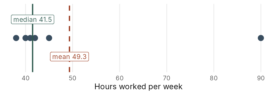
One extreme value pulls the mean (average) but not the median (middle value). Use the median when data are lopsided or have extreme values.
mean(students$Sleep, na.rm = TRUE)
median(students$Sleep, na.rm = TRUE)[1] 6.412414 [1] 6.5
The spread
sd(students$Sleep, na.rm = TRUE)
min(students$Sleep, na.rm = TRUE)
max(students$Sleep, na.rm = TRUE)
quantile(students$Sleep, probs = c(0.25, 0.75), na.rm = TRUE)
IQR(students$Sleep, na.rm = TRUE)[1] 0.8189691 [1] 4 [1] 9 25% 75% 5.9 6.9 [1] 1
- SD (standard deviation): the typical distance from the mean. Students sleep about 6.4 hours, give or take 0.8.
- IQR (interquartile range): the spread of the middle half. Goes with the median.
- Report mean + SD for symmetrical data, median + IQR for lopsided data.
One table per group
students %>%
  group_by(Gender) %>%
  summarise(n = n(),
            missing = sum(is.na(Sleep)),
            mean = mean(Sleep, na.rm = TRUE),
            sd = sd(Sleep, na.rm = TRUE),
            median = median(Sleep, na.rm = TRUE),
IQR = IQR(Sleep, na.rm = TRUE))# A tibble: 2 × 7 Gender n missing mean sd median IQR <chr> <int> <int> <dbl> <dbl> <dbl> <dbl> 1 Female 184 7 6.39 0.820 6.4 1.10 2 Male 116 3 6.45 0.820 6.5 1.1
Women and men sleep about the same.
Everything at once: describe()
library(psych)
students %>%
  select(Sleep, Stress, ExamScore) %>%
  describe()
vars n mean sd median trimmed mad min max range
Sleep 1 290 6.41 0.82 6.5 6.42 0.74 4 9 5
Stress 2 300 5.94 1.85 6.0 5.97 1.48 2 10 8
ExamScore 3 300 67.48 13.05 67.0 67.44 11.86 34 100 66
skew kurtosis se
Sleep -0.15 -0.09 0.05
Stress -0.10 -0.55 0.11
ExamScore 0.03 -0.08 0.75The key columns: n (non-missing), mean, sd, median, min, max, and skew (0 = symmetrical; between −1 and +1 is fine). The message when loading psych is normal.
Exercises
Describe exam scores
Find the mean, median, SD and IQR of ExamScore. Is it roughly symmetrical?
Show answerHide answer
mean(students$ExamScore)
median(students$ExamScore)
sd(students$ExamScore)
IQR(students$ExamScore)[1] 67.47667 [1] 67 [1] 13.05415 [1] 17
Mean (67.5) and median (67) are almost equal, so it's roughly symmetrical.
Compare groups
For each Motivation group: number of students, mean and SD of ExamScore, rounded to 1 decimal place. Show the groups in the order Low, Medium, High.
Show hintHide hint
Make Motivation a factor first (Lesson 7), then group_by() and summarise(). Wrap with round(..., 1).
Show answerHide answer
students %>%
  mutate(Motivation = factor(Motivation, levels = c("Low", "Medium", "High"))) %>%
  group_by(Motivation) %>%
  summarise(n = n(),
            mean = round(mean(ExamScore), 1),
sd = round(sd(ExamScore), 1))# A tibble: 3 × 4 Motivation n mean sd <fct> <int> <dbl> <dbl> 1 Low 66 58.7 11.7 2 Medium 147 67.7 12.2 3 High 87 73.7 11.7
describe()
Use describe() on Age, StudyHours and Attendance. Which is the most skewed? Why might that be?
Show answerHide answer
students %>% select(Age, StudyHours, Attendance) %>% describe() vars n mean sd median trimmed mad min max range
Age 1 300 21.09 1.99 21 20.88 1.48 18 29 11
StudyHours 2 294 14.07 5.98 14 14.13 5.93 0 31 31
Attendance 3 300 83.46 9.38 84 83.77 8.90 56 100 44
skew kurtosis se
Age 0.98 0.91 0.11
StudyHours -0.03 -0.32 0.35
Attendance -0.36 -0.12 0.54Age (skew 0.98): most students are 19 to 22, with a tail of a few older students.
Key points
- Middle: mean (with SD) or median (with IQR).
- Add
na.rm = TRUEwhen there are missing values, and reportn. describe()gives a full summary in one line.