Correlation | R for Psychological Research

Set up

R code

library(tidyverse)
students <- read_csv("data/students.csv", show_col_types = FALSE)

What r means

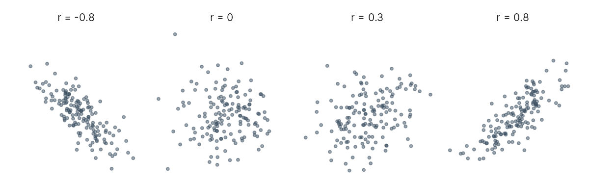
Four scatter plots with r of minus 0.8, 0, 0.3 and 0.8, from a tight falling band to a shapeless cloud to a tight rising band

r goes from −1 to +1.
Sign = direction: + both go up together; − one goes up as the other goes down.
Size = strength. Rough guide: .10 small, .30 medium, .50 large.

Plot first

R code

ggplot(students, aes(x = StudyHours, y = ExamScore)) +
  geom_point(alpha = 0.5) +
  geom_smooth(method = "lm")

Output

`geom_smooth()` using formula = 'y ~ x'
Warning messages:
1: Removed 6 rows containing non-finite outside the scale range
(`stat_smooth()`).
2: Removed 6 rows containing missing values or values outside the scale
range (`geom_point()`).

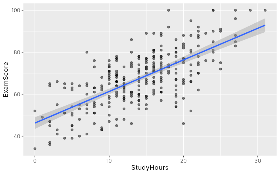
Scatter plot of study hours against exam score with a rising line

A clear rising pattern. The plot also shows if the pattern is curved or driven by a few odd points, which r alone can't tell you.

Calculate and test

R code

cor(students$StudyHours, students$ExamScore, use = "complete.obs")

Output

[1] 0.6892234

use = "complete.obs" skips students with a missing value. To test it:

R code

cor.test(students$StudyHours, students$ExamScore)

Output

	Pearson's product-moment correlation

data:  students$StudyHours and students$ExamScore
t = 16.255, df = 292, p-value < 2.2e-16
alternative hypothesis: true correlation is not equal to 0
95 percent confidence interval:
 0.6240309 0.7448873
sample estimates:
      cor 
0.6892234

cor = 0.69: a large positive correlation.
df = 292: students with both values (294) minus 2.
p-value < 2.2e-16: extremely small. Report as p < .001.
95% CI 0.62 to 0.74: where the true r probably lies.

Many at once

R code

students %>%
  select(StudyHours, Attendance, Sleep, Stress, ExamScore) %>%
  cor(use = "pairwise.complete.obs") %>%
  round(2)

Output

           StudyHours Attendance Sleep Stress ExamScore
StudyHours       1.00       0.14 -0.20   0.04      0.69
Attendance       0.14       1.00  0.12  -0.05      0.39
Sleep           -0.20       0.12  1.00  -0.30     -0.06
Stress           0.04      -0.05 -0.30   1.00     -0.01
ExamScore        0.69       0.39 -0.06  -0.01      1.00

Find a row and a column to read a pair. The diagonal is always 1.

Spearman's rho

For ratings (like stress, 1 to 10), skewed data or outliers, use Spearman's correlation. It uses ranks instead of raw values:

R code

cor.test(students$Stress, students$Sleep, method = "spearman")

Output

	Spearman's rank correlation rho

data:  students$Stress and students$Sleep
S = 5179207, p-value = 2.139e-06
alternative hypothesis: true rho is not equal to 0
sample estimates:
      rho 
-0.274165 
Warning message:
In cor.test.default(students$Stress, students$Sleep, method = "spearman") :
  Cannot compute exact p-value with ties

The warning about "ties" is normal for ratings. Report as r_s(288) = −.27, p < .001.

Correlation is not causation

A causes B?

More study → higher scores.

B causes A?

Doing well → enjoying study more.

C causes both?

Motivation → more study and higher scores.

A correlation can't tell these apart. Only an experiment can show cause and effect.

Exercises

Exercise 12.1 Dataset: students.csv

Attendance and exam

Plot Attendance against ExamScore, then test the correlation and report it.

Show answerHide answer

R code

ggplot(students, aes(x = Attendance, y = ExamScore)) +
  geom_point(alpha = 0.5) +
  geom_smooth(method = "lm")
cor.test(students$Attendance, students$ExamScore)

Output

`geom_smooth()` using formula = 'y ~ x'

	Pearson's product-moment correlation

data:  students$Attendance and students$ExamScore
t = 7.262, df = 298, p-value = 3.342e-12
alternative hypothesis: true correlation is not equal to 0
95 percent confidence interval:
 0.2871311 0.4799306
sample estimates:
      cor 
0.3877638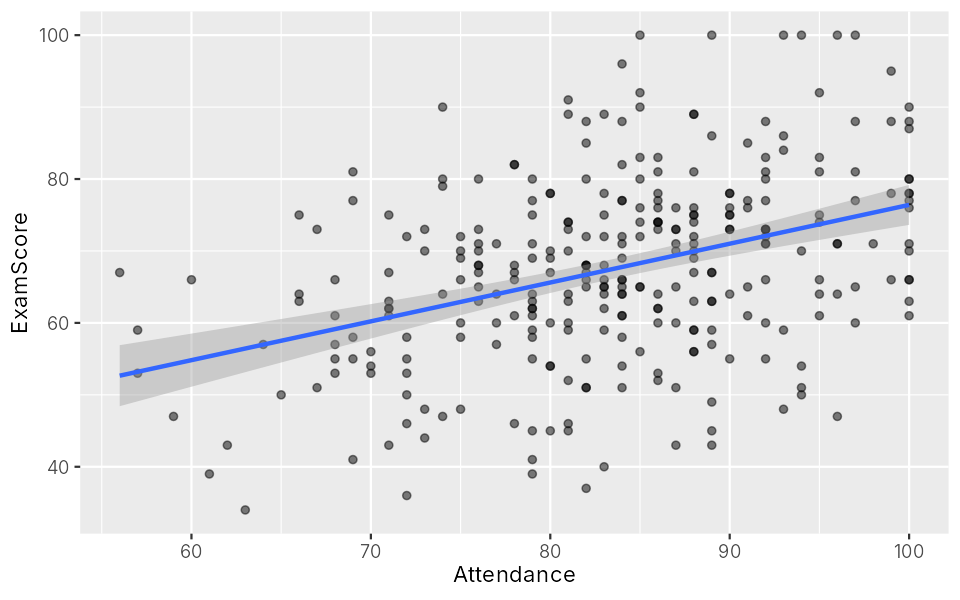

Scatter plot of attendance against exam score with a rising line

Attendance and exam scores were positively correlated, r(298) = .39, 95% CI [.29, .48], p < .001: a medium relationship.

Exercise 12.2 Dataset: students.csv

Sleep and stress

Test the (Pearson) correlation between Sleep and Stress. Is it positive or negative? Write the result.

Show answerHide answer

R code

cor.test(students$Sleep, students$Stress)

Output

	Pearson's product-moment correlation

data:  students$Sleep and students$Stress
t = -5.3437, df = 288, p-value = 1.854e-07
alternative hypothesis: true correlation is not equal to 0
95 percent confidence interval:
 -0.4016298 -0.1917994
sample estimates:
      cor 
-0.300344

Sleep and stress were negatively correlated, r(288) = −.30, 95% CI [−.40, −.19], p < .001. Students who sleep more tend to feel less stressed.

Exercise 12.3 Dataset: students.csv

A third variable?

Someone says: "Studying more causes higher grades." Using the data, show that motivation could explain part of the link.

Show hintHide hint

Compare study hours and exam scores across motivation groups with group_by() and summarise().

Show answerHide answer

R code

students %>%
  group_by(Motivation) %>%
  summarise(mean_study = mean(StudyHours, na.rm = TRUE), mean_exam = mean(ExamScore))

Output

# A tibble: 3 × 3
  Motivation mean_study mean_exam
  <chr>           <dbl>     <dbl>
1 High             17.2      73.7
2 Low              11.6      58.7
3 Medium           13.3      67.7

Motivated students both study more and score higher, so motivation could drive both.

Key points

Plot first, then cor.test().
Report r(df), the CI and p.
method = "spearman" for ratings or skewed data.
Correlation is not causation.