
Lesson 18 · Milestone
Milestone project
Bring lessons 0 to 17 together. Answer four research questions about the Student Life Survey on your own, from loading the data to writing the results.
The brief
The university wants four answers from the Student Life Survey. Use one script. Try each part before opening the answer, and use the Cheat sheet when stuck.
The steps of almost every analysis.
Describe the sample
Load the data. Report how many students there are, how many are female and male, their mean age (SD), and how many live in a hall or at home.
Show answerHide answer
library(tidyverse)
library(rstatix)
students <- read_csv("data/students.csv", show_col_types = FALSE)

students %>% summarise(n = n(), mean_age = mean(Age), sd_age = sd(Age))
students %>% count(Gender)
students %>% count(Living)
# A tibble: 1 × 3
n mean_age sd_age
<int> <dbl> <dbl>
1 300 21.1 1.99
# A tibble: 2 × 2
Gender n
<chr> <int>
1 Female 184
2 Male 116
# A tibble: 2 × 2
Living n
<chr> <int>
1 Hall 125
2 Home 175The sample was 300 students (184 female, 116 male), mean age 21.1 (SD = 2.0). 125 lived in a hall and 175 at home.
Question 1: sleep and stress
Do students who sleep less than 7 hours a night report more stress than those who sleep 7 hours or more?
Show hintHide hint
Make the two groups with mutate() and if_else(), then follow Lesson 15. Students with no sleep answer will get NA; drop them with drop_na().
Show answerHide answer
sleepers <- students %>%
  mutate(Sleep_Group = if_else(Sleep >= 7, "7 hours or more", "Under 7 hours")) %>%
  drop_na(Sleep_Group)

sleepers %>% group_by(Sleep_Group) %>% get_summary_stats(Stress, type = "mean_sd")
t_sleep <- sleepers %>% t_test(Stress ~ Sleep_Group)
t_sleep
sleepers %>% cohens_d(Stress ~ Sleep_Group)

ggplot(sleepers, aes(x = Sleep_Group, y = Stress)) +
  geom_boxplot() +
labs(x = NULL, y = "Stress (1 to 10)", subtitle = get_test_label(t_sleep, detailed = TRUE))# A tibble: 2 × 5 Sleep_Group variable n mean sd <chr> <fct> <dbl> <dbl> <dbl> 1 7 hours or more Stress 71 5.20 2.00 2 Under 7 hours Stress 219 6.19 1.70 # A tibble: 1 × 8 .y. group1 group2 n1 n2 statistic df p * <chr> <chr> <chr> <int> <int> <dbl> <dbl> <dbl> 1 Stress 7 hours or more Under 7 … 71 219 -3.76 105. 2.77e-4 # A tibble: 1 × 7 .y. group1 group2 effsize n1 n2 magnitude * <chr> <chr> <chr> <dbl> <int> <int> <ord> 1 Stress 7 hours or more Under 7 hours -0.534 71 219 moderate
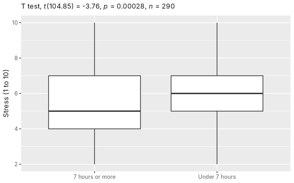
Students sleeping under 7 hours reported more stress (M = 6.19, SD = 1.70) than those sleeping 7 hours or more (M = 5.20, SD = 2.00), Welch's t(104.85) = 3.76, p < .001, d = 0.53.
Question 2: sleep and wellbeing
Is sleep related to wellbeing at the start of semester (Wellbeing_T1)?
Show answerHide answer
ggplot(students, aes(x = Sleep, y = Wellbeing_T1)) +
  geom_jitter(width = 0, height = 0.1, alpha = 0.4) +
  geom_smooth(method = "lm")
cor.test(students$Sleep, students$Wellbeing_T1)Warning messages: 1: Removed 10 rows containing non-finite outside the scale range (`stat_smooth()`). 2: Removed 10 rows containing missing values or values outside the scale range (`geom_point()`). Pearson's product-moment correlation data: students$Sleep and students$Wellbeing_T1 t = 3.2661, df = 288, p-value = 0.001222 alternative hypothesis: true correlation is not equal to 0 95 percent confidence interval: 0.07545037 0.29768727 sample estimates: cor 0.1889876
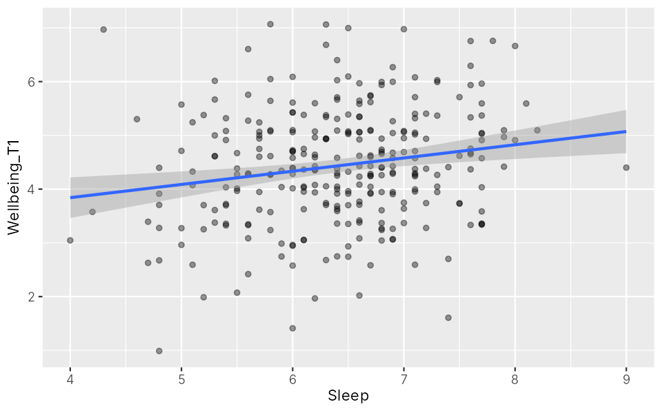
Sleep and wellbeing were weakly positively correlated, r(288) = .19, 95% CI [.08, .30], p = .001.
Question 3: hall life and the workshop
Were hall and home students equally likely to take the workshop?
Show answerHide answer
ws_living <- table(students$Living, students$Workshop)
prop.table(ws_living, margin = 1) %>% round(2)
chisq.test(ws_living)
cramer_v(ws_living)
         No  Yes
  Hall 0.59 0.41
  Home 0.61 0.39

	Pearson's Chi-squared test with Yates' continuity correction

data:  ws_living
X-squared = 0.014286, df = 1, p-value = 0.9049

[1] 0.01380131
Taking the workshop was not related to where students lived, χ²(1, N = 300) = 0.01, p = .905, V = .01 (41% of hall and 39% of home students took it).
Question 4: a chart for the report
Make one clear chart that shows how wellbeing changed for students with and without the workshop. Add a title and labels, and save it.
Show hintHide hint
Make Change = Wellbeing_T2 − Wellbeing_T1, then a boxplot of Change by Workshop. A dashed line at zero (geom_hline(yintercept = 0, linetype = "dashed")) shows "no change".
Show answerHide answer
students %>%
  mutate(Change = Wellbeing_T2 - Wellbeing_T1) %>%
  ggplot(aes(x = Workshop, y = Change)) +
  geom_hline(yintercept = 0, linetype = "dashed") +
  geom_boxplot(fill = "#FEF9E6") +
  labs(title = "Wellbeing rose for students who took the workshop",
       x = "Took the workshop", y = "Change in wellbeing (T2 - T1)") +
  theme_classic()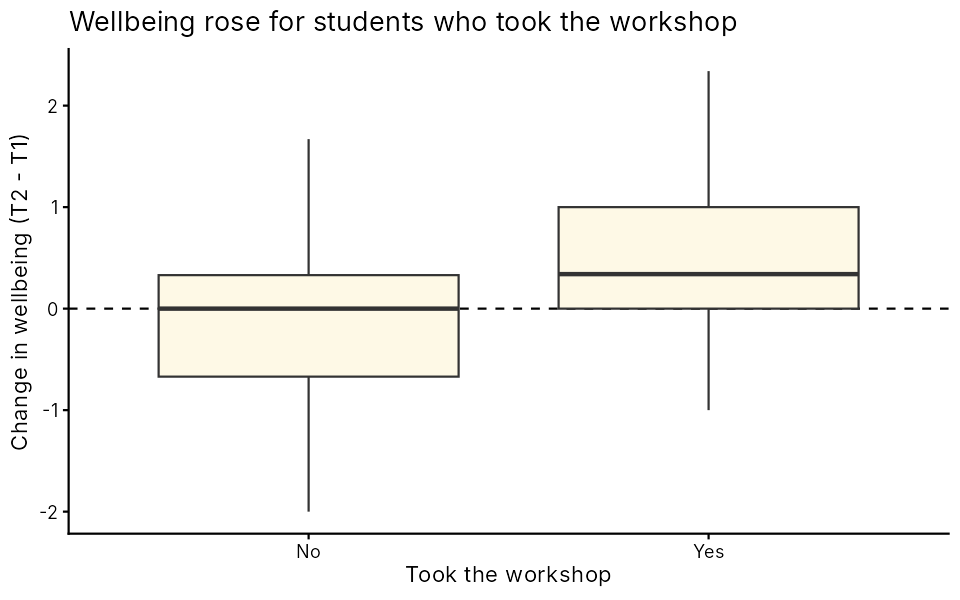
ggsave("workshop-change.png", width = 6, height = 4, dpi = 300)