z-scores

Set up

library(tidyverse)
students <- read_csv("data/students.csv", show_col_types = FALSE)

What a z-score means

A z-score is how far a score is from the mean, counted in SDs:

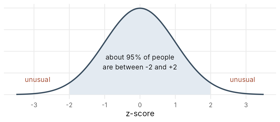
• z = 0: exactly average. z = 1: one SD above. z = −2: two SDs below.
• Beyond ±2 is unusual; beyond ±3 is rare.

Calculate z-scores

students <- students %>%
  mutate(z_Exam = (ExamScore - mean(ExamScore)) / sd(ExamScore))

students %>% select(ID, ExamScore, z_Exam) %>% head(4)

# A tibble: 4 × 3
  ID    ExamScore z_Exam
  <chr>     <dbl>  <dbl>
1 S001         73  0.423
2 S002         75  0.576
3 S003         52 -1.19 
4 S004         43 -1.88 

S004 scored 43: z = −1.88, nearly two SDs below average.

z-scores let you compare different scales. Is S005 more unusual in exam score (0 to 100) or stress (1 to 10)?

students <- students %>%
  mutate(z_Stress = (Stress - mean(Stress)) / sd(Stress))

students %>% filter(ID == "S005") %>% select(ID, ExamScore, z_Exam, Stress, z_Stress)

# A tibble: 1 × 5
  ID    ExamScore z_Exam Stress z_Stress
  <chr>     <dbl>  <dbl>  <dbl>    <dbl>
1 S005         88   1.57      7    0.573

S005's exam score (z = 1.57) is more unusual than their stress (z = 0.57).

Find unusual scores (abs() drops the minus sign):

students %>% filter(abs(z_Exam) > 2) %>% select(ID, ExamScore, z_Exam)

# A tibble: 16 × 3
   ID    ExamScore z_Exam
   <chr>     <dbl>  <dbl>
 1 S008         39  -2.18
 2 S084         39  -2.18
 3 S087         95   2.11
 4 S096         41  -2.03
 5 S102        100   2.49
 6 S109         36  -2.41
 7 S111        100   2.49
 8 S145         37  -2.33
 9 S165        100   2.49
10 S183         96   2.19
11 S218        100   2.49
12 S227         34  -2.56
13 S273         40  -2.10
14 S275        100   2.49
15 S297         41  -2.03
16 S298        100   2.49

One-sample z-test

Does a group's mean differ from a known population mean? You need the population's mean and SD.

Here, treat all 300 students as the population. Are mature students (aged 25 or over) more stressed than students in general?

mu <- mean(students$Stress)
sigma <- sd(students$Stress)
mature <- students %>% filter(Age >= 25)
nrow(mature)

[1] 20

library(BSDA)
z.test(x = mature$Stress, mu = mu, sigma.x = sigma)

Loading required package: lattice

Attaching package: ‘BSDA’

The following object is masked from ‘package:datasets’:

    Orange

	One-sample z-Test

data:  mature$Stress
z = -0.71094, p-value = 0.4771
alternative hypothesis: true mean is not equal to 5.943333
95 percent confidence interval:
 4.841315 6.458685
sample estimates:
mean of x 
     5.65 

• z = −0.71: the group mean is a little below the population mean.
• p = 0.477: not significant. No evidence that mature students differ.
• mean of x = 5.65: the mature students' average stress.

In real research you rarely know the population SD, so you'll usually use a t-test instead (Lessons 13 to 16). Same logic.

Exercises

students <- students %>%
  mutate(z_Sleep = (Sleep - mean(Sleep, na.rm = TRUE)) / sd(Sleep, na.rm = TRUE))
students %>% filter(abs(z_Sleep) > 2) %>% select(ID, Sleep, z_Sleep)

# A tibble: 9 × 3
  ID    Sleep z_Sleep
  <chr> <dbl>   <dbl>
1 S058    4.7   -2.09
2 S144    9      3.16
3 S176    4.6   -2.21
4 S177    4.7   -2.09
5 S217    8.1    2.06
6 S251    8.2    2.18
7 S261    4.3   -2.58
8 S269    4     -2.95
9 S287    4.2   -2.70

high <- students %>% filter(Motivation == "High")
z.test(x = high$ExamScore, mu = mean(students$ExamScore), sigma.x = sd(students$ExamScore))

	One-sample z-Test

data:  high$ExamScore
z = 4.4803, p-value = 7.453e-06
alternative hypothesis: true mean is not equal to 67.47667
95 percent confidence interval:
 71.00406 76.49020
sample estimates:
mean of x 
 73.74713 

Key points

• z = (score − mean) / SD. Beyond ±2 is unusual.
• z-scores compare variables on different scales.
• z.test(x, mu, sigma.x) (BSDA) compares a group with a known population.