Before a t-test | R for Psychological Research

Set up

R code

library(tidyverse)
library(rstatix)
library(pwr)
students <- read_csv("data/students.csv", show_col_types = FALSE)

The rstatix message about filter is normal.

Which t-test?

A t-test compares means.

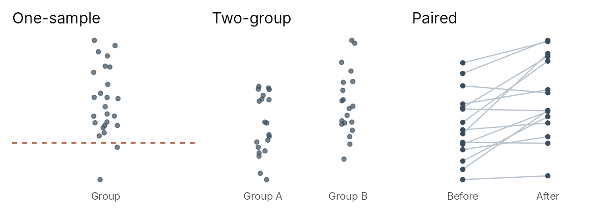
Three small charts. One-sample: one group of dots compared with a dashed line. Two groups: two separate groups of dots. Paired: the same people at two times, joined by lines

Test	Compares	Example (Lessons 14 to 16)
One-sample	one group's mean with a fixed value	Is wellbeing different from the scale midpoint, 4?
Two-group (independent)	two groups of different people	Do older and younger students differ?
Paired	the same people measured twice	Did wellbeing change from start to end of semester?

Plan the sample size: power

Power is the chance your study finds an effect that really exists. Aim for 80%. It depends on:

the effect size d (difference in SDs): 0.2 small, 0.5 medium, 0.8 large;
the significance level, usually .05;
the sample size, which you work out.

R code

pwr.t.test(d = 0.5, sig.level = .05, power = .80, type = "two.sample")

Output

     Two-sample t test power calculation 

              n = 63.76561
              d = 0.5
      sig.level = 0.05
          power = 0.8
    alternative = two.sided

NOTE: n is number in *each* group

n = 63.77, so round up: 64 people per group for a medium effect. For the other tests use type = "one.sample" or type = "paired" (both give 34).

Check the assumptions

1. Numbers

The outcome is numeric.

is.numeric()

2. Independent

Each person counted once, not influencing others. Comes from the study design.

3. No extreme outliers

identify_outliers(), boxplot

4. Roughly normal

shapiro_test(), Q-Q plot

R code

is.numeric(students$Wellbeing_T1)
students %>%
  identify_outliers(Wellbeing_T1) %>%
  select(ID, Wellbeing_T1, is.outlier, is.extreme)

Output

[1] TRUE
# A tibble: 8 × 4
  ID    Wellbeing_T1 is.outlier is.extreme
  <chr>        <dbl> <lgl>      <lgl>     
1 S002          1.33 TRUE       FALSE     
2 S035          7    TRUE       FALSE     
3 S179          7    TRUE       FALSE     
4 S194          7    TRUE       FALSE     
5 S239          7    TRUE       FALSE     
6 S246          1.67 TRUE       FALSE     
7 S261          7    TRUE       FALSE     
8 S263          1    TRUE       FALSE

Eight students count as outliers (very low scores or the top score, 7), but none is extreme (is.extreme is FALSE), and these are all possible answers on a 1 to 7 scale. They stay in.

Normality

R code

students %>% shapiro_test(Wellbeing_T1)
ggplot(students, aes(sample = Wellbeing_T1)) +
  stat_qq() +
  stat_qq_line()

Output

# A tibble: 1 × 3
  variable     statistic       p
  <chr>            <dbl>   <dbl>
1 Wellbeing_T1     0.987 0.00866

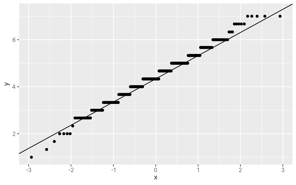
Q-Q plot where the points follow the straight line closely

Shapiro-Wilk: p < .05 suggests "not normal".
Q-Q plot: normal data follow the line.

Here p = .009, but the points hug the line. With large samples the test flags tiny differences that don't matter.

Exercises

Exercise 13.1 Dataset: students.csv

Which test?

Which t-test fits each question?

Do students who took the workshop differ in exam score from those who didn't?
Do students sleep less than the recommended 7 hours?
Did students' wellbeing change between T1 and T2?

Show answerHide answer

Two-group (different people in each group).
One-sample (one group against the value 7).
Paired (same people, twice).

Exercise 13.2 Dataset: students.csv

Power

How many students per group would you need to detect a large effect (d = 0.8) with a two-group t-test? And a small one (d = 0.2)?

Show answerHide answer

R code

pwr.t.test(d = 0.8, sig.level = .05, power = .80, type = "two.sample")
pwr.t.test(d = 0.2, sig.level = .05, power = .80, type = "two.sample")

Output

     Two-sample t test power calculation 

              n = 25.52458
              d = 0.8
      sig.level = 0.05
          power = 0.8
    alternative = two.sided

NOTE: n is number in *each* group


     Two-sample t test power calculation 

              n = 393.4057
              d = 0.2
      sig.level = 0.05
          power = 0.8
    alternative = two.sided

NOTE: n is number in *each* group

26 per group for a large effect, but 394 per group for a small one.

Exercise 13.3 Dataset: students.csv

Check Sleep

Check Sleep for extreme outliers and normality.

Show answerHide answer

R code

students %>% identify_outliers(Sleep) %>% select(ID, Sleep, is.outlier, is.extreme)
students %>% shapiro_test(Sleep)
ggplot(students, aes(sample = Sleep)) + stat_qq() + stat_qq_line()

Output

# A tibble: 4 × 4
  ID    Sleep is.outlier is.extreme
  <chr> <dbl> <lgl>      <lgl>     
1 S144    9   TRUE       FALSE     
2 S261    4.3 TRUE       FALSE     
3 S269    4   TRUE       FALSE     
4 S287    4.2 TRUE       FALSE     
# A tibble: 1 × 3
  variable statistic     p
  <chr>        <dbl> <dbl>
1 Sleep        0.993 0.221
Warning messages:
1: Removed 10 rows containing non-finite outside the scale range
(`stat_qq()`).
2: Removed 10 rows containing non-finite outside the scale range
(`stat_qq_line()`).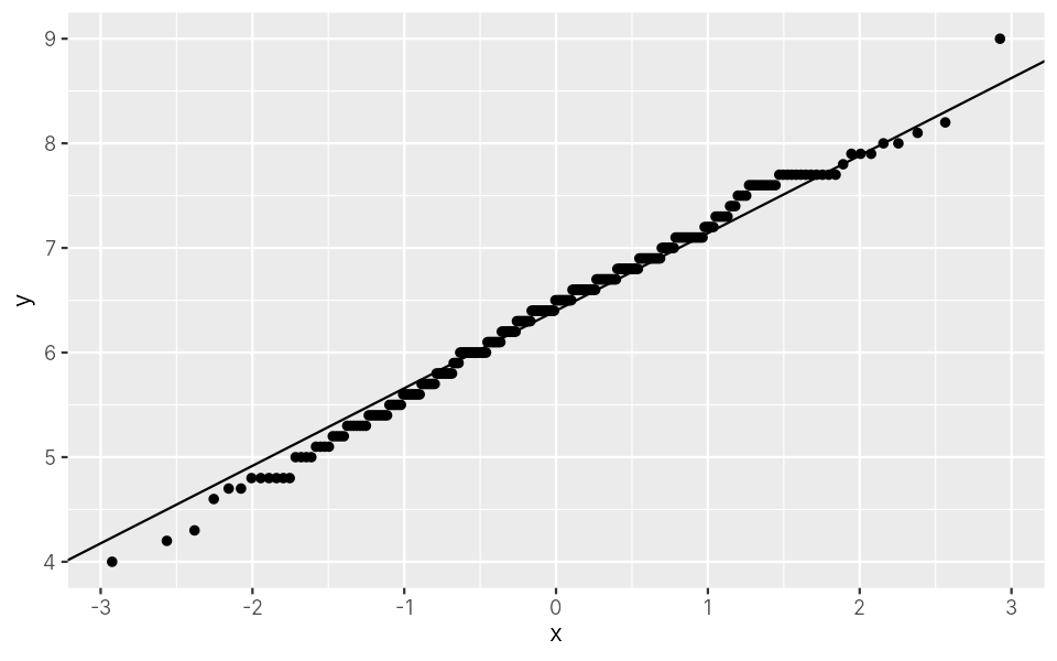

Q-Q plot of sleep with points close to the line

Four students are outliers but none is extreme, and the Shapiro-Wilk test is not significant (p = .22), so Sleep looks normal.

Key points

One-sample: vs a value. Two-group: different people. Paired: same people twice.
pwr.t.test() gives the sample size. Round up.
Check outliers and normality; with 30+ per group, small departures are fine.