Two-group t-test | R for Psychological Research

Set up

R code

library(tidyverse)
library(rstatix)
students <- read_csv("data/students.csv", show_col_types = FALSE) %>%
  mutate(Age_Group = if_else(Age >= 21, "21 and over", "Under 21"))

Age_Group splits students into two groups (Lesson 6).

The question

Do older students (21 and over) have different wellbeing at the start of semester from younger students?

Describe and check

R code

students %>%
  group_by(Age_Group) %>%
  get_summary_stats(Wellbeing_T1, type = "mean_sd")

Output

# A tibble: 2 × 5
  Age_Group   variable         n  mean    sd
  <chr>       <fct>        <dbl> <dbl> <dbl>
1 21 and over Wellbeing_T1   159  4.59  1.05
2 Under 21    Wellbeing_T1   141  4.26  1.03

Both groups have well over 30 students, so normality is not a worry (Lesson 13).

Run the test

Wellbeing_T1 ~ Age_Group means "wellbeing, split by age group". Save the result to use in a chart:

R code

t_age <- students %>% t_test(Wellbeing_T1 ~ Age_Group)
t_age
students %>% cohens_d(Wellbeing_T1 ~ Age_Group)

Output

# A tibble: 1 × 8
  .y.          group1      group2     n1    n2 statistic    df       p
* <chr>        <chr>       <chr>   <int> <int>     <dbl> <dbl>   <dbl>
1 Wellbeing_T1 21 and over Under …   159   141      2.78  295. 0.00586
# A tibble: 1 × 7
  .y.          group1      group2   effsize    n1    n2 magnitude
* <chr>        <chr>       <chr>      <dbl> <int> <int> <ord>    
1 Wellbeing_T1 21 and over Under 21   0.321   159   141 small

t = 2.78, p = .006: significant.
The df has decimals because R uses Welch's t-test, which doesn't assume equal spreads in the two groups. It's the safe default.
Positive t: group1 ("21 and over") has the higher mean.
d = 0.32: a small effect.

Show it

get_test_label() turns the result into a chart subtitle:

R code

ggplot(students, aes(x = Age_Group, y = Wellbeing_T1)) +
  geom_boxplot() +
  labs(subtitle = get_test_label(t_age, detailed = TRUE),
       x = "Age group", y = "Wellbeing at T1 (1 to 7)")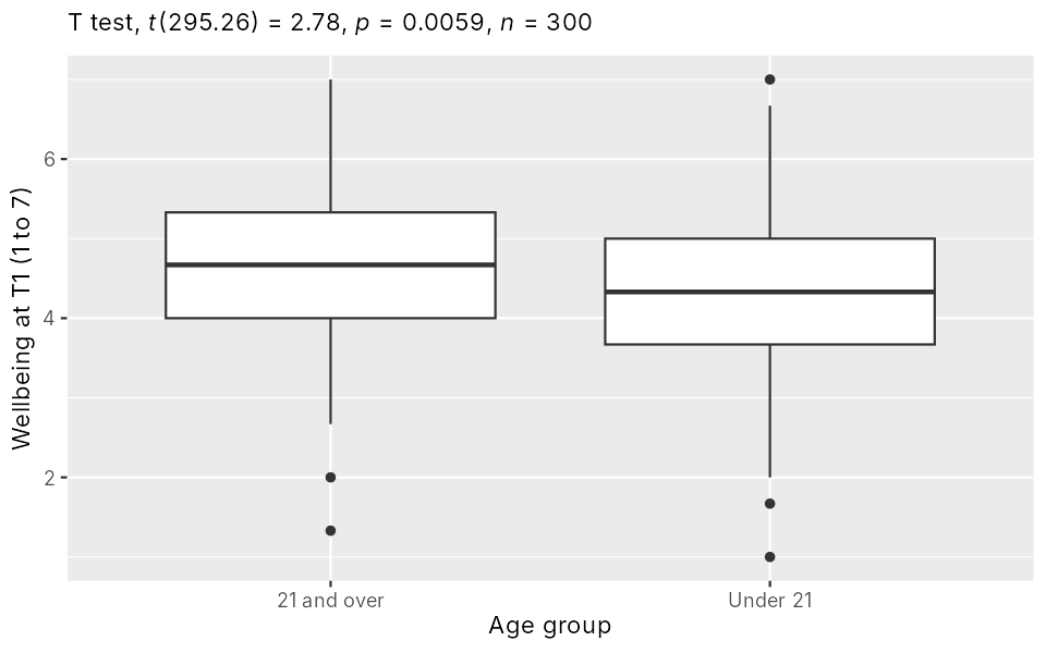

Boxplots of wellbeing for the two age groups, with the t-test result as the subtitle; the 21 and over box is slightly higher

Exercises

Exercise 15.1 Dataset: students.csv

Did the workshop help?

Some students took a wellbeing workshop during the semester (Workshop).

Create Change = Wellbeing_T2 − Wellbeing_T1.
Get the mean and SD of Change for each Workshop group.
Compare them with a t-test, get Cohen's d, and make a boxplot with the result.
Report it.

Show hintHide hint

mutate() first. Then the same steps as this lesson, with Change ~ Workshop.

Show answerHide answer

R code

students <- students %>% mutate(Change = Wellbeing_T2 - Wellbeing_T1)

students %>%
  group_by(Workshop) %>%
  get_summary_stats(Change, type = "mean_sd")

t_ws <- students %>% t_test(Change ~ Workshop)
t_ws
students %>% cohens_d(Change ~ Workshop)

ggplot(students, aes(x = Workshop, y = Change)) +
  geom_boxplot() +
  labs(subtitle = get_test_label(t_ws, detailed = TRUE),
       x = "Took the workshop", y = "Change in wellbeing")

Output

# A tibble: 2 × 5
  Workshop variable     n   mean    sd
  <chr>    <fct>    <dbl>  <dbl> <dbl>
1 No       Change     180 -0.182 0.676
2 Yes      Change     120  0.493 0.698
# A tibble: 1 × 8
  .y.    group1 group2    n1    n2 statistic    df        p
* <chr>  <chr>  <chr>  <int> <int>     <dbl> <dbl>    <dbl>
1 Change No     Yes      180   120     -8.30  250. 6.57e-15
# A tibble: 1 × 7
  .y.    group1 group2 effsize    n1    n2 magnitude
* <chr>  <chr>  <chr>    <dbl> <int> <int> <ord>    
1 Change No     Yes     -0.981   180   120 large

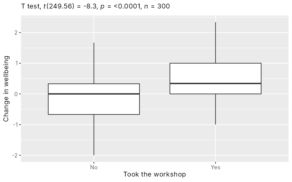
Boxplots of wellbeing change: the workshop group is above zero, the no-workshop group slightly below

Students who took the workshop improved more (M = 0.49, SD = 0.70) than those who didn't (M = −0.18, SD = 0.68), Welch's t(249.56) = 8.30, p < .001, d = 0.98: a large effect. The t is negative only because "No" comes first.

Exercise 15.2 Dataset: students.csv

Hall or home?

Do students living in a hall and at home differ in Stress? Report it, including when the result is not significant.

Show answerHide answer

R code

students %>% group_by(Living) %>% get_summary_stats(Stress, type = "mean_sd")
students %>% t_test(Stress ~ Living)
students %>% cohens_d(Stress ~ Living)

Output

# A tibble: 2 × 5
  Living variable     n  mean    sd
  <chr>  <fct>    <dbl> <dbl> <dbl>
1 Hall   Stress     125  5.82  2.02
2 Home   Stress     175  6.03  1.71
# A tibble: 1 × 8
  .y.    group1 group2    n1    n2 statistic    df     p
* <chr>  <chr>  <chr>  <int> <int>     <dbl> <dbl> <dbl>
1 Stress Hall   Home     125   175    -0.921  239. 0.358
# A tibble: 1 × 7
  .y.    group1 group2 effsize    n1    n2 magnitude 
* <chr>  <chr>  <chr>    <dbl> <int> <int> <ord>     
1 Stress Hall   Home    -0.109   125   175 negligible

Not significant: hall and home students reported similar stress. A non-significant result means no clear evidence of a difference, not proof that there is none.

Key points

t_test(outcome ~ group) compares two groups (Welch's test by default).
cohens_d() for the effect size; get_test_label() for the chart.
Report both groups' M and SD, then t(df), p, d.