Chi-square test | R for Psychological Research

Set up

R code

library(tidyverse)
library(rstatix)
students <- read_csv("data/students.csv", show_col_types = FALSE) %>%
  mutate(LearningStyle = case_when(
    LearningStyle == 0 ~ "Visual",
    LearningStyle == 1 ~ "Kinaesthetic",
    LearningStyle == 2 ~ "Auditory",
    LearningStyle == 3 ~ "Reading/Writing"
  ))

When to use it

When both variables are categories, there are no means to compare, only counts. Question: does preferred learning style differ between female and male students?

H0: the two are unrelated. H1: they are related.
The test compares the counts you observed with the counts you'd expect if H0 were true.

Count

R code

style_table <- table(students$Gender, students$LearningStyle)
style_table

Output

        
         Auditory Kinaesthetic Reading/Writing Visual
  Female       29           39              50     66
  Male         19           22              30     45

Groups differ in size (184 women, 116 men), so compare percentages within each row:

R code

prop.table(style_table, margin = 1) %>% round(2)

Output

        
         Auditory Kinaesthetic Reading/Writing Visual
  Female     0.16         0.21            0.27   0.36
  Male       0.16         0.19            0.26   0.39

The percentages are very similar for women and men.

R code

ggplot(students, aes(x = Gender, fill = LearningStyle)) +
  geom_bar(position = "fill") +
  labs(y = "Proportion", fill = "Learning style")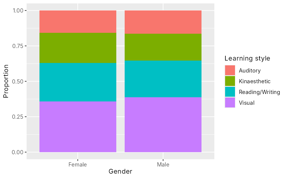

Proportion bars for female and male students, split into four learning styles in nearly the same proportions

position = "fill" stretches each bar to full height, so you compare proportions.

Test

R code

chi <- chisq.test(style_table)
chi

Output

	Pearson's Chi-squared test

data:  style_table
X-squared = 0.4013, df = 3, p-value = 0.94

X-squared = χ² = 0.40: a tiny gap between observed and expected.
df = (rows − 1) × (columns − 1) = 1 × 3 = 3.
p = 0.94: not significant.

Check: expected counts of 5 or more

R code

chi$expected

Output

        
         Auditory Kinaesthetic Reading/Writing Visual
  Female    29.44     37.41333        49.06667  68.08
  Male      18.56     23.58667        30.93333  42.92

All above 5, so the test is valid. If any were below 5, use fisher.test(style_table).

Effect size: Cramér's V

R code

cramer_v(style_table)

Output

[1] 0.03657392

From 0 (no link) to 1. Rough guide: .10 small, .30 medium, .50 large. Here, almost 0.

Exercises

Exercise 17.1 Dataset: students.csv

Hall life and support

Are students who live in a hall more or less likely to use the university's wellbeing support (Used_Support)?

Make the table and row percentages.
Draw a proportion bar chart.
Run the chi-square test, check the expected counts, and get Cramér's V.
Report it.

Show answerHide answer

R code

support_table <- table(students$Living, students$Used_Support)
support_table
prop.table(support_table, margin = 1) %>% round(2)

ggplot(students, aes(x = Living, fill = Used_Support)) +
  geom_bar(position = "fill") +
  labs(y = "Proportion", fill = "Used support")

chi2 <- chisq.test(support_table)
chi2
chi2$expected
cramer_v(support_table)

Output

      
        No Yes
  Hall  82  43
  Home 137  38
      
         No  Yes
  Hall 0.66 0.34
  Home 0.78 0.22

	Pearson's Chi-squared test with Yates' continuity correction

data:  support_table
X-squared = 5.3272, df = 1, p-value = 0.02099

      
           No   Yes
  Hall  91.25 33.75
  Home 127.75 47.25
[1] 0.1408719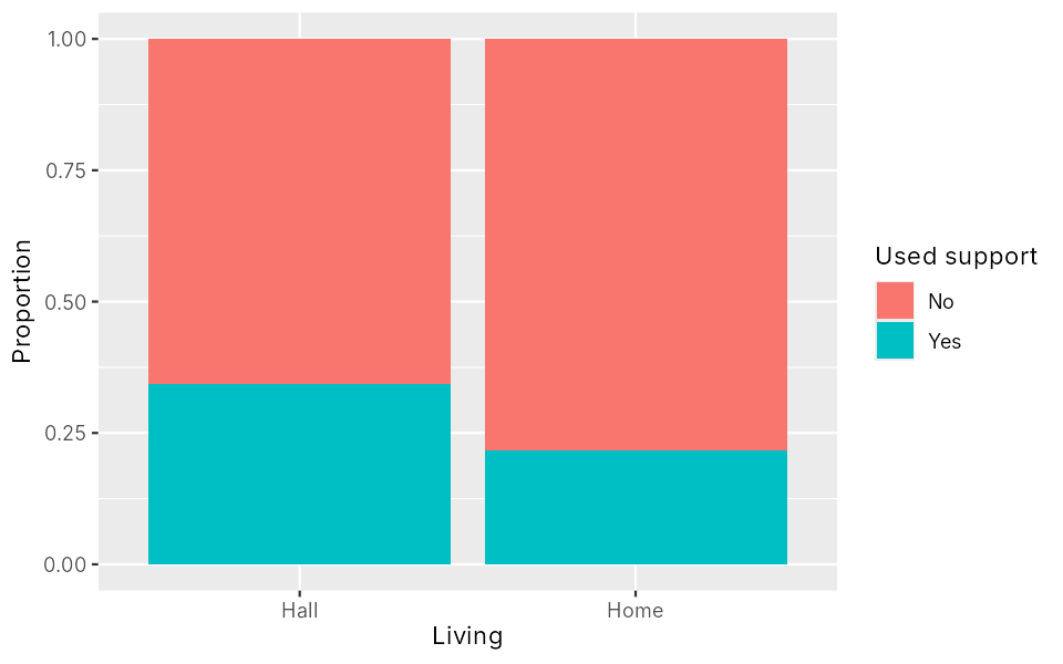

Proportion bars: a larger share of hall students used support than home students

Hall students were more likely to use wellbeing support (34%) than students living at home (22%), χ²(1, N = 300) = 5.33, p = .021, V = .14. For a 2 × 2 table R applies Yates' continuity correction, a small adjustment that makes the test a little more cautious.

Exercise 17.2 Dataset: students.csv

Workshop and gender

Is taking the workshop related to gender? Run the test and report it.

Show answerHide answer

R code

ws_table <- table(students$Gender, students$Workshop)
prop.table(ws_table, margin = 1) %>% round(2)
chisq.test(ws_table)
cramer_v(ws_table)

Output

        
           No  Yes
  Female 0.55 0.45
  Male   0.67 0.33

	Pearson's Chi-squared test with Yates' continuity correction

data:  ws_table
X-squared = 3.655, df = 1, p-value = 0.0559

[1] 0.1173642

Not significant, though close: χ²(1, N = 300) = 3.66, p = .056, V = .12. A p just above .05 is still not significant; report the exact value and let readers judge.

Key points

Two categorical variables: chi-square test.
table() for counts, prop.table(margin = 1) for row percentages.
Check $expected is at least 5; otherwise fisher.test().
Report χ²(df, N), p and Cramér's V.